This web page is intended to serve as a guide procedures to install the MPAS-JEDI at EGEON.
Exercises are split into seven main sections, each of which focuses on
a particular aspect of using the MPAS-JEDI data assimilation system.
In case you would like to refer to any of the lecture slides from previous days,
you can open the Tutorial Agenda in another window.
The test dataset can be downloaded from Here.
You can proceed through the sections of this practical guide at your own pace. It is highly recommended
to go through the exercises in order, since later exercises may require the output of earlier ones.
Clicking the grey headers will expand each section or subsection.
The practical exercises in this tutorial have been tailored to work on
the Egeon system.
Egeon is a Dell EMC cluster that provides most of the libraries needed by MPAS-JEDI and its pre- and post-processing tools through modules. In general, before compiling and running MPAS-JEDI on your own system,
you will need to install spack-stack.
However, this tutorial does not cover the installation of spack-stack, which was pre-installed on Egeon.
MPAS-JEDI code build for this tutorial is based upon the develop branch of spack-stack, close to version spack-stack-1.7.0.
Logging onto Egeon from your laptop or desktop by
$ ssh -X username@egeon-login.cptec.inpe.br
then using your password to get onto Egeon. Note that
'-X' is necessary in order to use X11-forwarding for direct graphics display from Egeon.
It is recommened to at least login onto Egeon with two terminals for different tasks.
It is assumed that each user should be under bash after logging in, use "echo $SHELL"
to double check.
First, copy the pre-prepared tutorial test dataset directory to your own beegfs disk space:
$ cd /mnt/beegfs/${USER}
$ cp -r /mnt/beegfs/professor/mpasjedi_tutorial/mpasjedi_tutorial2024_testdata ./mpas_jedi_tutorial
$ ls -l mpas_jedi_tutorial

total 7
drwxr-sr-x 3 professor professor   1 Aug  7 19:40 background
drwxr-sr-x 3 professor professor   1 Aug  7 19:36 background_120km
drwxr-sr-x 5 professor professor   3 Aug  7 19:39 B_Matrix
drwxr-sr-x 4 professor professor  38 Aug  9 06:18 conus15km
drwxr-sr-x 2 professor professor  27 Aug  7 19:36 crtm_coeffs_v3
drwxr-sr-x 3 professor professor   1 Aug  7 19:36 ensemble
drwxr-sr-x 2 professor professor 168 Aug  7 19:36 localization_pregenerated
drwxr-sr-x 2 professor professor  35 Aug 10 00:59 MPAS_JEDI_yamls_scripts
drwxr-sr-x 2 professor professor  30 Aug  8 04:13 MPAS_namelist_stream_physics_files
drwxr-sr-x 2 professor professor   6 Aug  7 19:40 ncl_scripts
drwxrwsr-x 5 professor professor   7 Aug  9 21:58 obs2ioda_prebuild
drwxr-sr-x 3 professor professor   7 Aug  8 19:11 obs_bufr
drwxr-sr-x 3 professor professor   1 Aug  7 19:35 obs_ioda_pregenerated
drwxr-sr-x 4 professor professor   2 Aug  9 00:41 omboma_from2experiments
This copy will take some time as the size of the whole directory is ~16GB!
You may pay special attention to the following directories:
- obs2ioda_prebuild - Pre-build bufr2ioda converter as a backup plan in case you fail to compile it yourself.
- obs_ioda_pregenerated - Pre-converted ioda obs as a backup plan in case you fail the obs conversion exercise.
- localization_pregenerated - Pre-generated BUMP localization files
as a backup plan in case you fail the localization generation exercise.
Egeon uses the LMOD package to manage the software development.
Run module list to see what modules are loaded by default
right after you log in.
It should print something similar to below:
$ module list

Currently Loaded Modules:
  1) autotools   2) prun/2.2   3) gnu9/9.4.0   4) hwloc/2.5.0   5) ucx/1.11.2   6) libfabric/1.13.0   7) openmpi4/4.1.1   8) ohpc
Post-processing and graphics exercises will need Python and NCAR Command
Language (NCL).
On Egeon, these are available in
a Conda environment named 'mpasjedi'. The 'mpasjedi' environment also provides
NCL. We can load the Anaconda module and activate the 'mpasjedi' environment with
the following commands:
$ module load anaconda3-2022.05-gcc-11.2.0-q74p53i
$ source "/opt/spack/opt/spack/linux-rhel8-zen2/gcc-11.2.0/anaconda3-2022.05-q74p53iarv7fk3uin3xzsgfmov7rqomj/etc/profile.d/conda.sh"
$ conda activate /mnt/beegfs/professor/conda/envs/mpasjedi
$ module load imagemagick-7.0.8-7-gcc-11.2.0-46pk2go
$ which ncl # check whether ncl exists
You will run all of the practical exercises in your own beegfs space under
/mnt/beegfs/${USER}/mpas_jedi_tutorial.
Running jobs on Egeon requires the submission of a job script to a batch queueing system,
which will allocate requested computing resources to your job when they become available.
In general, it's best to avoid running any compute-intensive jobs on the login nodes, and
the practical instructions to follow will guide you in the process of submitting jobs when
necessary.
As a first introduction to running jobs on Egeon, there are several key commands worth
noting:
- sbatch job-script - This command submits a slurm job script, which describes a job
to be run on one or more batch nodes.
- squeue -u ${USER} - This command tells you the status of your pending and running jobs.
Note that you may need to wait about 30 seconds for a recently submitted job to show up.
- scancel JobID - This command deletes a queued or running job
Throughout this tutorial, you will submit your jobs to the batch partition queue. At various points in the practical exercises, we'll need to submit jobs to Egeon's queueing system
using the sbatch command, and after doing so, we may often check on the status
of the job with the squeue command, monitoring the log files produced by the job
once we see that the job has begun to run. Most exercises will run with 64 cores of one single node
though each of Egeon's nodes have 128 cores (512GB available memory).
Note that 4DEnVar uses 3 nodes with the analyses at 3 times.
You're now ready to begin with the practical exercises of this tutorial!
In this section, the goal is to obtain, compile, and test the MPAS-JEDI code
through cmake/ctest mechanism. It is much important beggiing a new prompt using the egeon-Login1. For this enter again in the egeon.
Logging onto Egeon-login1 from your laptop or desktop by
$ ssh -X username@egeon-login1
In order to build MPAS-JEDI and its dependencies, it is recommended to access source code from mpas-bundle.
However, to save time for this tutorial, we will use a 'local' version of source code and test dataset, which correspons to the 'release/3.0.0-beta' branch from mpas-bundle-3.0.0-beta:
$ cd /mnt/beegfs/${USER}/mpas_jedi_tutorial
$ cp /mnt/beegfs/professor/mpasjedi_tutorial/mpasbundlev3_local.tar.gz .
$ tar xzf mpasbundlev3_local.tar.gz
$ ls -l mpasbundlev3_local/*
You will see
mpasbundlev3_local/build:
total 1
drwxrwsr-x 3 professor professor 1 Aug 13 21:15 test_data

mpasbundlev3_local/code:
total 34
-rw-rw-r--  1 professor professor  5032 Aug 13 21:28 CMakeLists.txt
drwxrwsr-x 11 professor professor    21 Aug 13 21:08 crtm
drwxrwsr-x  2 professor professor     7 Aug 14 08:58 env-setup
drwxrwsr-x 10 professor professor    18 Aug 13 21:09 ioda
drwxrwsr-x  5 professor professor     5 Aug 13 21:12 ioda-data
-rw-rw-r--  1 professor professor 11334 Aug 13 21:09 LICENSE
drwxrwsr-x  8 professor professor    12 Aug 13 21:09 MPAS
drwxrwsr-x 11 professor professor    17 Aug 13 21:09 mpas-jedi
drwxrwsr-x  4 professor professor     8 Aug 13 23:35 mpas-jedi-data
drwxrwsr-x 13 professor professor    23 Aug 13 21:08 oops
-rw-rw-r--  1 professor professor 10146 Aug 13 21:09 README.md
drwxrwsr-x 12 professor professor    22 Aug 13 21:12 saber
drwxrwsr-x  2 professor professor     2 Aug 13 21:10 scripts
drwxrwsr-x  3 professor professor     2 Aug 13 21:12 test-data-release
drwxrwsr-x 11 professor professor    19 Aug 13 21:10 ufo
drwxrwsr-x  6 professor professor     7 Aug 13 23:58 ufo-data
drwxrwsr-x  9 professor professor    14 Aug 13 21:12 vader
One important difference from previous mpas-bundle releases (1.0.0 and 2.0.0) is
that 3.0.0-based bundle works together with the official 8.2.x-based MPAS-A model code from
https://github.com/MPAS-Dev/MPAS-Model/tree/hotfix-v8.2.1, instead of 7.x-based code
from https://github.com/JCSDA-internal/MPAS-Model.
We now enter the 'build' folder, run the script build_pyjedi.sh to install pyjedi in the /mnt/beegfs/${USER}/jedi. Note that is necessary deactivate the base conda environment:
$  cd mpasbundlev3_local/build
$  conda deactivate
$  /mnt/beegfs/jose.aravequia/jedi/build_pyjedi.sh
After load the spack-stack environment pre-built by Aravequia
using the IFORT compiler and list the available modules. For this copy the script edited by any user and run it:
$  cp /home/luiz.sapucci/bin/SpackStackAraveck_intel_env_mpas_v8.2 .
$  . /mnt/beegfs/${USER}/mpas_jedi_tutorial/mpasbundlev3_local/build/SpackStackAraveck_intel_env_mpas_v8.2
$  module list
The output to the module list in the terminal should look like the following.
These packages are from pre-installed spack-stack.
 Currently Loaded Modules:
  1) tbb/2021.4.0                    10) jedi-intel/2021.4.0  19) hdf5/1.12.0           28) cgal/5.0.4                   37) gmp/6.2.1
  2) compiler-rt/2021.4.0            11) mpi/2021.4.0         20) pnetcdf/1.12.1        29) fftw/3.3.8                   38) mpfr/4.2.1
  3) debugger/2021.6.0               12) impi/2021.4.0        21) netcdf/4.9.2          30) bufr/noaa-emc-12.0.0         39) lapack/3.8.0
  4) dpl/2021.4.0                    13) jedi-impi/2021.4.0   22) nccmp/1.8.7.0         31) pybind11/2.11.0              40) git-lfs/2.11.0
  5) oclfpga/2021.4.0                14) ecbuild/ecmwf-3.8.4  23) eckit/ecmwf-1.24.4    32) gsl_lite/0.37.0              41) ecflow/5.5.3
  6) curl-7.85.0-gcc-11.2.0-yxw2lyk  15) cmake/3.30.2         24) fckit/ecmwf-0.11.0    33) pio/2.6.2-debug              42) python-3.9.15-gcc-9.4.0-f466wuv
  7) compiler/2021.4.0               16) szip/2.1.1           25) atlas/ecmwf-0.36.0    34) json/3.9.1                   43) esmf/v8.6.0
  8) intel/2021.4.0                  17) udunits/2.2.28       26) boost-headers/1.68.0  35) json-schema-validator/2.1.0  44) fms/jcsda-release-stable
  9) mkl/2021.4.0                    18) zlib/1.2.11          27) eigen/3.4.0           36) odc/ecmwf-1.5.2
Check if your ${bundle_dir} variable is correct pointing for your jedi diretory, like is showed bellow.
$  echo ${bundle_dir}
/mnt/beegfs/${USER}/mpas_jedi_tutorial/mpasbundlev3_local
$
If yes, now we are ready to compile actual source code through cmake and make.
MPAS-JEDI uses cmake to automatically download the code from various github repositories,
listed in CMakeLists.txt under ~code. Now type the command below under the build directory:
$ cmake ../code
Note that the CMakeLists.txt file under "../code" was modified for this tutorial so that cmake will NOT fetch
code and test data from github, instead, it uses the pre-downloaded local code/testdata under "../code".
After cmake completes (5 min or so),
"Makefile" files to build executables are generated under the build directory.
Now it is ready to compile MPAS-JEDI under 'build' using the standard make. For this practice, we will compile the code on the login node, but in the future, consider compiling code
using a compute node with an interactive job or by submitting a job to a computing node.
$ make -j18
This could take ~25 min. Using more cores for build could speed up a bit, but will not help too much from our experience.
WARNING:The compilation could take ~25 min to complet. You may continue to read instructions while waiting.
Once we reach 100% of the compilation, many executables will be generated under ~build/bin.
MPAS-A model and MPAS-JEDI DA related executables are:
$ ls bin/mpas*
bin/mpas_atmosphere                     bin/mpasjedi_enshofx.x                   bin/mpasjedi_rtpp.x
bin/mpas_atmosphere_build_tables        bin/mpasjedi_ens_mean_variance.x         bin/mpasjedi_saca.x
bin/mpas_init_atmosphere                bin/mpasjedi_error_covariance_toolbox.x  bin/mpasjedi_variational.x
bin/mpasjedi_convertstate.x             bin/mpasjedi_forecast.x                  bin/mpas_namelist_gen
bin/mpasjedi_converttostructuredgrid.x  bin/mpasjedi_gen_ens_pert_B.x            bin/mpas_parse_atmosphere
bin/mpasjedi_eda.x                      bin/mpasjedi_hofx3d.x                    bin/mpas_parse_init_atmosphere
bin/mpasjedi_enkf.x                     bin/mpasjedi_hofx.x                      bin/mpas_streams_gen
The last step is to ensure that the code was compiled properly by running the MPAS-JEDI ctests,
with two lines of simple command:
$ export LD_LIBRARY_PATH=/mnt/beegfs/${USER}/mpas_jedi_tutorial/mpasbundlev3_local/build/lib:$LD_LIBRARY_PATH
$ cd mpas-jedi
$ ctest
At the moment the tests are running (take ~4 min to finish), it indicates if it passes or fails.
At the end, a summary is provided with a percentage of the tests that passed, failed and the processing times.
The output to the terminal should look as following:
......

98% tests passed, 1 tests failed out of 56

Label Time Summary:
executable    =  99.22 sec*proc (13 tests)
mpasjedi      = 532.14 sec*proc (56 tests)
mpi           = 525.55 sec*proc (55 tests)
script        = 432.92 sec*proc (43 tests)

Total Test time (real) = 532.84 sec

The following tests FAILED:
          2 - test_mpasjedi_geometry (Failed)
Errors while running CTest
Output from these tests are in: /mnt/beegfs/$USER/mpas_jedi_tutorial/mpasbundlev3_local/build/mpas-jedi/Testing/Temporary/LastTest.log
Use "--rerun-failed --output-on-failure" to re-run the failed cases verbosely.
Idealy, you should see all 57 ctest cases pass. However, 1 cases of using more than 1 core are failing on Egeon
for some unknow reason. This will not affect usage of JEDI at EGEON.
WARNING:You could run ctest just under the 'build' directory, but that will run a total of 2111 ctest cases for all
component packages (oops, vader, saber, ufo, ioda, crtm, mpas-jedi etc.) in mpas-bundle, which will take much longer time.
Maybe something you could play out of this tutorial.
To determine if a test passes or fails, a comparison of the test log and reference file is done internally taking as reference a tolerance value. This tolerance is specified via YAML file. These files can be found under mpas-jedi/test/testoutput in the build folder:
3denvar_2stream_bumploc.ref       4denvar_ID.run                          ens_mean_variance.run.ref
3denvar_2stream_bumploc.run       4denvar_ID.run.ref                      forecast.ref
3denvar_2stream_bumploc.run.ref   4denvar_VarBC_nonpar.run                forecast.run
3denvar_amsua_allsky.ref          4denvar_VarBC_nonpar.run.ref            forecast.run.ref
3denvar_amsua_allsky.run          4denvar_VarBC.ref                       gen_ens_pert_B.ref
3denvar_amsua_allsky.run.ref      4denvar_VarBC.run                       gen_ens_pert_B.run
3denvar_amsua_bc.ref              4denvar_VarBC.run.ref                   gen_ens_pert_B.run.ref
3denvar_amsua_bc.run              4dfgat.ref                              hofx3d_nbam.ref
3denvar_amsua_bc.run.ref          4dfgat.run                              hofx3d_nbam.run
3denvar_bumploc.ref               4dfgat.run.ref                          hofx3d_nbam.run.ref
3denvar_bumploc.run               4dhybrid_bumpcov_bumploc.ref            hofx3d.ref
3denvar_bumploc.run.ref           4dhybrid_bumpcov_bumploc.run            hofx3d_ropp.ref
3denvar_dual_resolution.ref       4dhybrid_bumpcov_bumploc.run.ref        hofx3d_rttovcpp.ref
3denvar_dual_resolution.run       convertstate_bumpinterp.ref             hofx3d.run
3denvar_dual_resolution.run.ref   convertstate_bumpinterp.run             hofx3d.run.ref
3dfgat_pseudo.ref                 convertstate_bumpinterp.run.ref         hofx4d_pseudo.ref
3dfgat_pseudo.run                 convertstate_unsinterp.ref              hofx4d_pseudo.run
3dfgat_pseudo.run.ref             convertstate_unsinterp.run              hofx4d_pseudo.run.ref
3dfgat.ref                        convertstate_unsinterp.run.ref          hofx4d.ref
3dfgat.run                        converttostructuredgrid_latlon.ref      hofx4d.run
3dfgat.run.ref                    converttostructuredgrid_latlon.run      hofx4d.run.ref
3dhybrid_bumpcov_bumploc.ref      converttostructuredgrid_latlon.run.ref  letkf_3dloc.ref
3dhybrid_bumpcov_bumploc.run      dirac_bumpcov.ref                       letkf_3dloc.run
3dhybrid_bumpcov_bumploc.run.ref  dirac_bumpcov.run                       letkf_3dloc.run.ref
3dvar_bumpcov_nbam.ref            dirac_bumpcov.run.ref                   lgetkf_height_vloc.ref
3dvar_bumpcov_nbam.run            dirac_bumploc.ref                       lgetkf_height_vloc.run
3dvar_bumpcov_nbam.run.ref        dirac_bumploc.run                       lgetkf_height_vloc.run.ref
3dvar_bumpcov.ref                 dirac_bumploc.run.ref                   lgetkf.ref
3dvar_bumpcov_ropp.ref            dirac_noloc.ref                         lgetkf.run
3dvar_bumpcov_rttovcpp.ref        dirac_noloc.run                         lgetkf.run.ref
3dvar_bumpcov.run                 dirac_noloc.run.ref                     parameters_bumpcov.ref
3dvar_bumpcov.run.ref             dirac_spectral_1.ref                    parameters_bumpcov.run
3dvar.ref                         dirac_spectral_1.run                    parameters_bumpcov.run.ref
3dvar.run                         dirac_spectral_1.run.ref                parameters_bumploc.ref
3dvar.run.ref                     eda_3dhybrid.ref                        parameters_bumploc.run
4denvar_bumploc.ref               eda_3dhybrid.run                        parameters_bumploc.run.ref
4denvar_bumploc.run               eda_3dhybrid.run.ref                    rtpp.ref
4denvar_bumploc.run.ref           ens_mean_variance.ref                   rtpp.run
4denvar_ID.ref                    ens_mean_variance.run                   rtpp.run.ref
Tutorial attendees should use this pre-build bundle for mpas-jedi practices and should
set an environment variable 'bundle_dir' for convenience in the subsequent practicals.
$ export bundle_dir=/mnt/beegfs/$USER/mpasjedi_tutorial/mpas_bundle_v3
The goal of this session is to create the observation input files needed for running
subsequent MPAS-JEDI test cases.
First, navigate to the mpas_jedi_tutorial directory and create a directory for converting NCEP BUFR observations to IODA-HDF5 format. Then, clone the obs2ioda repository and proceed with compiling the converter.
$ cd /mnt/beegfs/${USER}/mpas_jedi_tutorial
$ git clone https://github.com/NCAR/obs2ioda
$ cd obs2ioda/obs2ioda-v2/src/
$ source ../../../obs2ioda_prebuild/obs2ioda-env.sh
To compile the converter, you need the NCEP BUFR library (available at https://github.com/NOAA-EMC/NCEPLIBS-bufr) along with the netcdf-c and netcdf-fortran libraries. Depending on how netcdf is configured on your system, the C and Fortran bindings may be installed in different directories. To verify their locations, use the following commands:
$ nc-config --prefix
$ nf-config --prefix
On Egeon, the netcdf-c and netcdf-fortran libraries are installed in separate directories. Their paths are stored in environment variables: NETCDF_FORTRAN_INC, NETCDF_FORTRAN_LIB, NETCDF_INCLUDE, and NETCDF_LIB. For efficiency, we will use a precompiled version of the NCEPLIBS-bufr library located in:
/mnt/beegfs/${USER}/mpas_jedi_tutorial/obs2ioda_prebuild/NCEPLIBS-bufr
Next, locate the NCEPLIBS-bufr library directory using the find utility:
$ find /mnt/beegfs/${USER}/mpas_jedi_tutorial/obs2ioda_prebuild/NCEPLIBS-bufr -name "*libbufr*"
Copy the preconfigured Makefile into the obs2ioda source directory and rerun make.
$ cp ../../../obs2ioda_prebuild/Makefile .
Finally, compile the converter using the make command:
$  make clean
$  make
If the compilation is successful, the executable obs2ioda-v2.x will be generated.
The NCEP bufr input files are under the existing ~obs_bufr folder. Now we need to convert
the bufr-format data into the ioda-hdf5 format under the ~obs_ioda folder.
$ mkdir /mnt/beegfs/${USER}/mpas_jedi_tutorial/obs_ioda
$ cd /mnt/beegfs/${USER}/mpas_jedi_tutorial/obs_ioda
$ mkdir 2018041500
$ cd 2018041500
The next commands from section 2.2, 2.3 and 2.4 can be executed using the scripts comandos.ksh. Copy this script and running it. Press "enter to continuin and "n" to stop the process"
$ cp /mnt/beegfs/luiz.sapucci/mpas_jedi_tutorial/obs_ioda/2018041500/comandos.ksh .
$  ./comandos.ksh
Case you is not able to use this script, you should do the step-by-step below. Link the prepbufr/bufr files to the working directory:
$ ln -fs ../../obs_bufr/2018041500/prepbufr.gdas.20180415.t00z.nr.48h .
$ ln -fs ../../obs_bufr/2018041500/gdas.1bamua.t00z.20180415.bufr .
$ ln -fs ../../obs_bufr/2018041500/gdas.gpsro.t00z.20180415.bufr .
$ ln -fs ../../obs_bufr/2018041500/gdas.satwnd.t00z.20180415.bufr .
Link executables and files:
$ ln -fs ../../obs2ioda/obs2ioda-v2/src/obs2ioda-v2.x .
$ ln -fs ${bundle_dir}/build/bin/ioda-upgrade-v1-to-v2.x .
$ ln -fs ${bundle_dir}/build/bin/ioda-upgrade-v2-to-v3.x .
$ ln -fs ${bundle_dir}/code/env-setup/gnu-egeon.csh .
$ ln -fs ${bundle_dir}/code/ioda/share/ioda/yaml/validation/ObsSpace.yaml .
Copy obs_errtable to work directory:
$ cp ../../obs_bufr/2018041500/obs_errtable .
Now we can run obs2ioda-v2.x.
The usage is:
$ ./obs2ioda-v2.x [-i input_dir] [-o output_dir] [bufr_filename(s)_to_convert]
If input_dir and output_dir are not specified, the default is the current working directory.
If bufr_filename(s)_to_convert is not specified, the code looks for file name, **prepbufr.bufr** (also **satwnd.bufr**, **gnssro.bufr**, **amsua.bufr**, **airs.bufr**, **mhs.bufr**, **iasi.bufr**, **cris.bufr**) in the input/working directory. If the file exists, do the conversion, otherwise skip it.
$ ./obs2ioda-v2.x prepbufr.gdas.20180415.t00z.nr.48h
$ ./obs2ioda-v2.x gdas.satwnd.t00z.20180415.bufr
$ ./obs2ioda-v2.x gdas.gpsro.t00z.20180415.bufr
$ ./obs2ioda-v2.x gdas.1bamua.t00z.20180415.bufr
Create the directory iodav2
and move amsua and gnssro h5 files to the directory iodav2.
$ mkdir iodav2
$ mv amsua_*obs* iodav2
$ mv gnssro_obs_*.h5  iodav2
Due to NetCDF-Fortran interface does not allow reading/writing NF90_STRING, so station_id and variable_names are still written out as
char station_id(nlocs, nstring)
char variable_names(nvars, nstring)
rather than
string station_id(nlocs)
string variable_names(nvars)
So, for aircraft/satwind/satwnd/sfc/sondes, we need run upgrade executable ioda-upgrade-v1-to-v2.x.
The output files for aircraft/satwind/satwnd/sfc/sondes are created in iodav2 directory.
The input *h5 files in currect directory can be deleted.
$ source ${bundle_dir}/code/env-setup/gnu-egeon.sh
$ ./ioda-upgrade-v1-to-v2.x satwind_obs_2018041500.h5 iodav2/satwind_obs_2018041500.h5
$ ./ioda-upgrade-v1-to-v2.x satwnd_obs_2018041500.h5 iodav2/satwnd_obs_2018041500.h5
$ ./ioda-upgrade-v1-to-v2.x sfc_obs_2018041500.h5 iodav2/sfc_obs_2018041500.h5
$ ./ioda-upgrade-v1-to-v2.x aircraft_obs_2018041500.h5 iodav2/aircraft_obs_2018041500.h5
$ ./ioda-upgrade-v1-to-v2.x sondes_obs_2018041500.h5 iodav2/sondes_obs_2018041500.h5
$ rm *.h5
Now we can convert iodav2 to iodav3 format by using ioda-upgrade-v2-to-v3.x. Remember to load the spack-stack modules for Egeon before executing the IODA upgraders.
$ source ${bundle_dir}/code/env-setup/gnu-egeon.sh
$ ./ioda-upgrade-v2-to-v3.x iodav2/aircraft_obs_2018041500.h5 ./aircraft_obs_2018041500.h5 ObsSpace.yaml
$ ./ioda-upgrade-v2-to-v3.x iodav2/gnssro_obs_2018041500.h5 ./gnssro_obs_2018041500.h5 ObsSpace.yaml
$ ./ioda-upgrade-v2-to-v3.x iodav2/satwind_obs_2018041500.h5 ./satwind_obs_2018041500.h5 ObsSpace.yaml
$ ./ioda-upgrade-v2-to-v3.x iodav2/satwnd_obs_2018041500.h5 ./satwnd_obs_2018041500.h5 ObsSpace.yaml
$ ./ioda-upgrade-v2-to-v3.x iodav2/sfc_obs_2018041500.h5 ./sfc_obs_2018041500.h5 ObsSpace.yaml
$ ./ioda-upgrade-v2-to-v3.x iodav2/sondes_obs_2018041500.h5 ./sondes_obs_2018041500.h5 ObsSpace.yaml
$ ./ioda-upgrade-v2-to-v3.x iodav2/amsua_n15_obs_2018041500.h5 ./amsua_n15_obs_2018041500.h5 ObsSpace.yaml
$ ./ioda-upgrade-v2-to-v3.x iodav2/amsua_n18_obs_2018041500.h5 ./amsua_n18_obs_2018041500.h5 ObsSpace.yaml
$ ./ioda-upgrade-v2-to-v3.x iodav2/amsua_n19_obs_2018041500.h5 ./amsua_n19_obs_2018041500.h5 ObsSpace.yaml
$ ./ioda-upgrade-v2-to-v3.x iodav2/amsua_metop-a_obs_2018041500.h5 ./amsua_metop-a_obs_2018041500.h5 ObsSpace.yaml
$ ./ioda-upgrade-v2-to-v3.x iodav2/amsua_metop-b_obs_2018041500.h5 ./amsua_metop-b_obs_2018041500.h5 ObsSpace.yaml
Now you have the proper format ioda files under ~obs_ioda/2018041500 for subsequent mpas-jedi tests:
aircraft_obs_2018041500.h5       amsua_n18_obs_2018041500.h5  satwnd_obs_2018041500.h5
amsua_metop-a_obs_2018041500.h5  amsua_n19_obs_2018041500.h5  sfc_obs_2018041500.h5
amsua_metop-b_obs_2018041500.h5  gnssro_obs_2018041500.h5     sondes_obs_2018041500.h5
amsua_n15_obs_2018041500.h5      satwind_obs_2018041500.h5
Setup conda environment for plotting.
Note that we need to load the conda environment before executing the Python script.
If you have already loaded the spack-stack modules, please open a new prompt before loading the conda environment 'mpasjedi'. The important is that the spack-stack has not been loaded to use the mpasjedi env.
$  ssh -X username@egeon-login.cptec.inpe.br
$ cd /mnt/beegfs/${USER}/mpas_jedi_tutorial/obs_ioda/2018041500
$ module load anaconda3-2022.05-gcc-11.2.0-q74p53i
$ source "/opt/spack/opt/spack/linux-rhel8-zen2/gcc-11.2.0/anaconda3-2022.05-q74p53iarv7fk3uin3xzsgfmov7rqomj/etc/profile.d/conda.sh"
$ conda activate /mnt/beegfs/professor/conda/envs/mpasjedi
An additional step is needed for satellite radiance data (e.g, amsua_n15, amsua_metop-a) in order to convert the 'sensorScanPosition' variable from float point to integer. This is a requirement after changes for consistency between in UFO and IODA. For this, we have prepared the script 'run_updateSensorScanPosition.csh' that will link fix_float2int.py and update_sensorScanPosition.py, set environment variables, and execute the Python scripts.
$ ln -sf ../../MPAS_JEDI_yamls_scripts/run_updateSensorScanPosition.csh
$ ./run_updateSensorScanPosition.csh
To check that radiance files have been updated, run ncdump and check for the variable 'sensorScanPosition' under the 'Metadata' group.
$ source ../../obs2ioda_prebuild/obs2ioda-env.sh
$ ncdump -h amsua_n15_obs_2018041500.h5
Or simply run:
$ source ../../obs2ioda_prebuild/obs2ioda-env.sh
$ ncdump -h amsua_n15_obs_2018041500.h5 | grep sensorScanPosition
TO generate the figures, copy graphics directory to current directory:
$ cp -r ${bundle_dir}/code/mpas-jedi/graphics .
$ cd graphics/standalone
Edit the line 80 of the python plot_obs_loc_tut.py script and put there as is showed here
"channels = ObsSpaceInfo.get('channels',[vu.miss_i])", and after save this changing.
Due to some unknown problem to plot metob-b amsu data, and need move it to another extention, so it do not break other plots.
$ mv ../../amsua_metop-b_obs_2018041500.h5 ../../amsua_metop-b_obs_2018041500.h5.notplotable
Now, run the script calling the python:
$ python plot_obs_loc_tut.py
Now, one of the figures shown here:
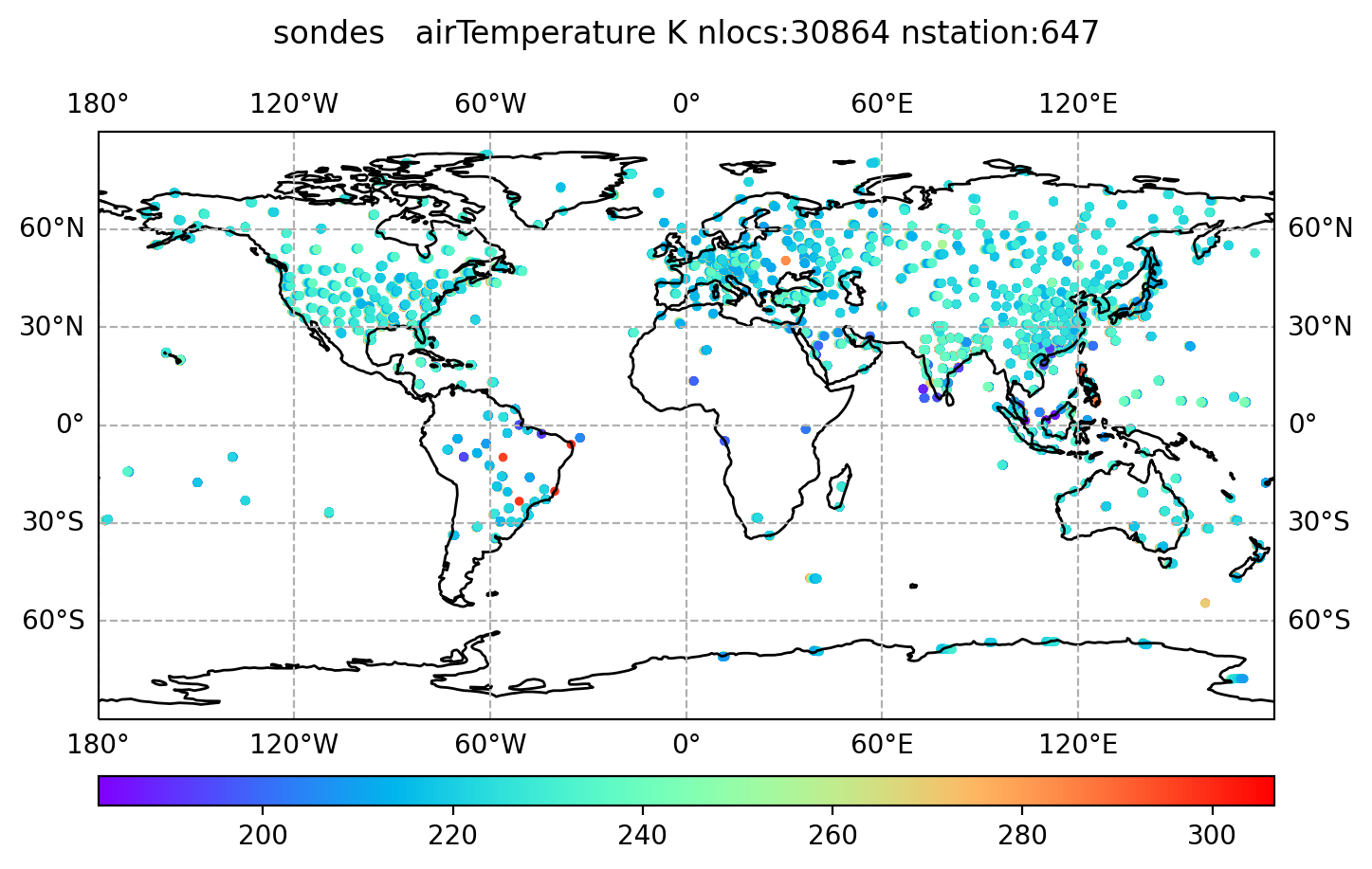
$ module load imagemagick-7.0.8-7-gcc-11.2.0-46pk2go
$ display distri_airTemperature_sondes_obs_2018041500_all.png

In this session, we will be running an application called 𝐻(𝐱).
Creating hofx directory in mpas_jedi_tutorial,
$ cd /mnt/beegfs/${USER}/mpas_jedi_tutorial
$ mkdir hofx
$ cd hofx
Certifify that the enviroment variable is pointed by your mpas-bundle directory, giving the source the Spack-Stack-Araveck
$ . /mnt/beegfs/${USER}/mpas_jedi_tutorial/mpasbundlev3_local/build/SpackStackAraveck_intel_env_mpas_v8.2
The next commands in this section to prepare the environment can be executed using the scripts commandos.ksh. Copy this script and running it.
$ cp /mnt/beegfs/luiz.sapucci/mpas_jedi_tutorial/hofx/comandos.ksh .
$  ./comandos.ksh
Proceed to the next section, but case you is not able to use this script, you should do the step-by-step below in this section.
The following commands are for linking files, such as,
physics-related data and tables, MPAS graph, streams, and namelist files:
$ ln -fs ../MPAS_namelist_stream_physics_files/*TBL .
$ ln -fs ../MPAS_namelist_stream_physics_files/*DBL .
$ ln -fs ../MPAS_namelist_stream_physics_files/*DATA .
$ ln -fs ../MPAS_namelist_stream_physics_files/x1.10242.graph.info.part.64 .
$ ln -fs ../MPAS_namelist_stream_physics_files/namelist.atmosphere_240km .
$ ln -fs ../MPAS_namelist_stream_physics_files/streams.atmosphere_240km .
$ ln -fs ../MPAS_namelist_stream_physics_files/stream_list.atmosphere.analysis .
$ ln -fs ../MPAS_namelist_stream_physics_files/stream_list.atmosphere.background .
$ ln -fs ../MPAS_namelist_stream_physics_files/stream_list.atmosphere.control .
$ ln -fs ../MPAS_namelist_stream_physics_files/stream_list.atmosphere.ensemble .
Link yamls:
$ ln -fs ${bundle_dir}/code/mpas-jedi/test/testinput/namelists/geovars.yaml .
$ ln -fs ${bundle_dir}/code/mpas-jedi/test/testinput/namelists/keptvars.yaml .
$ ln -fs ${bundle_dir}/code/mpas-jedi/test/testinput/obsop_name_map.yaml .
Link MPAS 6-h forecast background file into template file and an MPAS invariant file for 2-stream I/O:
$ ln -fs ../MPAS_namelist_stream_physics_files/x1.10242.invariant.nc .
$ ln -fs ../background/2018041418/mpasout.2018-04-15_00.00.00.nc templateFields.10242.nc
Link the background and observation input files:
$ ln -fs ../background/2018041418/mpasout.2018-04-15_00.00.00.nc ./bg.2018-04-15_00.00.00.nc
$ ln -fs ../obs_ioda_pregenerated/2018041500/aircraft_obs_2018041500.h5  .
$ ln -fs ../obs_ioda_pregenerated//2018041500/gnssro_obs_2018041500.h5  .
$ ln -fs ../obs_ioda_pregenerated/2018041500/satwind_obs_2018041500.h5  .
$ ln -fs ../obs_ioda_pregenerated/2018041500/sfc_obs_2018041500.h5  .
$ ln -fs ../obs_ioda_pregenerated/2018041500/sondes_obs_2018041500.h5  .
Copy hofx3d.yaml and run_hofx3d.csh to the working directory:
$ ln -sf ../MPAS_JEDI_yamls_scripts/hofx3d.yaml .
Several experiencies indicated that the Spack Stack should be loaded before to sumit the job. The enverioment will be sent to the core and is not
necessary to give the source in the script to load the Spack Stack. This script is commented. The $bundle_dir is exported and some change it is need
to do some changes in the submit file run_hofx3d.csh: change the partition to PESQ2, the name of the job. In ordem to make easear this task,
it is suggested see our copy the file indicated bellow.
$ cp /mnt/beegfs/luiz.sapucci/mpas_jedi_tutorial/hofx/MPAS_JEDI_yamls_scripts/run_hofx3d.csh .
Certifify that the SpackStackAraveck is loaded and after submit a SLURM job to run hofx,
$  . /mnt/beegfs/${USER}/mpas_jedi_tutorial/mpasbundlev3_local/build/SpackStackAraveck_intel_env_mpas_v8.2
$  sbatch run_hofx3d.csh
According to the setting in hofx3d.yaml, the output files are obsout_hofx_*.h5.
You may check the output file content using 'ncdump -h obsout_hofx_aircraft.h5'.
you can also check hofx by running python.
Setup conda environment for plotting.
Note that we need to load the conda environment before executing the Python script.
If you have already loaded the spack-stack modules, please open a new prompt before loading the conda environment 'mpasjedi'. The important is that the spack-stack has not been loaded to use the mpasjedi env.
$  ssh -X username@egeon-login.cptec.inpe.br
$ cd /mnt/beegfs/${USER}/mpas_jedi_tutorial/hofx
$ module load anaconda3-2022.05-gcc-11.2.0-q74p53i
$ source "/opt/spack/opt/spack/linux-rhel8-zen2/gcc-11.2.0/anaconda3-2022.05-q74p53iarv7fk3uin3xzsgfmov7rqomj/etc/profile.d/conda.sh"
$ conda activate /mnt/beegfs/professor/conda/envs/mpasjedi
The following steps are for set up python enviorment, copy graphics directory, and run plot_diag.py:
$ cp -r ${bundle_dir}/code/mpas-jedi/graphics .
$ cd graphics/standalone
$ python plot_diag.py
This will produce a number of figure files, display of one of them
$ module load imagemagick-7.0.8-7-gcc-11.2.0-46pk2go
$ display distri_windEastward_hofx_aircraft_omb_allLevels.png
which will look like the figure below

To view more figures, it is more convenent to transfer them to your local computer via:
$ scp -r ${USER}@egeon-login.cptec.inpe.br:/mnt/beegfs/${USER}/mpas_jedi_tutorial/hofx/graphics/standalone .
In this practice, we will generate the BUMP localization files to be used for spatial localization
of ensemble background error covariance. These files will be used in the following 3D/4DEnVar and hybrid-3DEnVar
data assimilation practice.
After changing to our /mnt/beegfs/${USER}/mpas_jedi_tutorial directory,
create the working directory.
$ cd /mnt/beegfs/${USER}/mpas_jedi_tutorial
$ mkdir localization
$ cd localization
Certifify that the enviroment variable is pointed by your mpas-bundle directory, giving the source the Spack-Stack-Araveck
$ . /mnt/beegfs/${USER}/mpas_jedi_tutorial/mpasbundlev3_local/build/SpackStackAraveck_intel_env_mpas_v8.2
The next commands in this section to prepare the environment can be executed using the scripts commandos.ksh. Copy this script and running it.
$ cp /mnt/beegfs/luiz.sapucci/mpas_jedi_tutorial/localization/comandos.ksh .
$  ./comandos.ksh
Check and subit the sumit-file, but case you is not able to use this script, you should do the step-by-step below in this section.
Link MPAS physics-related data and tables, MPAS graph, MPAS streams, MPAS namelist files.
$ ln -fs ../MPAS_namelist_stream_physics_files/*BL ./
$ ln -fs ../MPAS_namelist_stream_physics_files/*DATA ./
$ ln -fs ../MPAS_namelist_stream_physics_files/x1.10242.graph.info.part.64 ./
$ ln -fs ../MPAS_namelist_stream_physics_files/streams.atmosphere_240km ./
$ ln -fs ../MPAS_namelist_stream_physics_files/stream_list.atmosphere.analysis ./
$ ln -fs ../MPAS_namelist_stream_physics_files/stream_list.atmosphere.background ./
$ ln -fs ../MPAS_namelist_stream_physics_files/stream_list.atmosphere.control ./
$ ln -fs ../MPAS_namelist_stream_physics_files/stream_list.atmosphere.ensemble ./
$ ln -fs ../MPAS_namelist_stream_physics_files/namelist.atmosphere_240km ./
Link MPAS 2-stream files.
$ ln -fs ../background/2018041418/mpasout.2018-04-15_00.00.00.nc ./
$ ln -fs ../background/2018041418/mpasout.2018-04-15_00.00.00.nc ./templateFields.10242.nc
$ ln -fs ../MPAS_namelist_stream_physics_files/x1.10242.invariant.nc .
Link yaml files.
$ ln -fs ${bundle_dir}/code/mpas-jedi/test/testinput/namelists/geovars.yaml  ./
$ ln -fs ${bundle_dir}/code/mpas-jedi/test/testinput/namelists/keptvars.yaml  ./
$ ln -fs ../MPAS_JEDI_yamls_scripts/bumploc.yaml ./
Copy the SLURM job script.
$ cp ../MPAS_JEDI_yamls_scripts/run_bumploc.csh ./
It is need change the path of the $bundle_dir and comment the line to install Spack Stack, because is not necessary, and partition to PESQ2 in the submit file run_bumploc.csh. In ordem to make easear this task copy this file as indicated bellow.
$ cp /mnt/beegfs/luiz.sapucci/mpas_jedi_tutorial/localization/run_bumploc.csh .
Certifify that the SpackStackAraveck is loaded and after submit a SLURM job to run hofx,
$  . /mnt/beegfs/${USER}/mpas_jedi_tutorial/mpasbundlev3_local/build/SpackStackAraveck_intel_env_mpas_v8.2
$  sbatch run_bumploc.csh
User may check the SLURM job status by running squeue -u ${USER},
or monitoring the log file jedi.log.
After finishing the SLURM job, user can check the BUMP localization files generated. The "local" files are generated for each processor (64 processors in this practice).
$ ls bumploc_1200km6km_nicas_local_*.nc

bumploc_1200km6km_nicas_local_000064-000001.nc  bumploc_1200km6km_nicas_local_000064-000033.nc
bumploc_1200km6km_nicas_local_000064-000002.nc  bumploc_1200km6km_nicas_local_000064-000034.nc
bumploc_1200km6km_nicas_local_000064-000003.nc  bumploc_1200km6km_nicas_local_000064-000035.nc
bumploc_1200km6km_nicas_local_000064-000004.nc  bumploc_1200km6km_nicas_local_000064-000036.nc
bumploc_1200km6km_nicas_local_000064-000005.nc  bumploc_1200km6km_nicas_local_000064-000037.nc
bumploc_1200km6km_nicas_local_000064-000006.nc  bumploc_1200km6km_nicas_local_000064-000038.nc
bumploc_1200km6km_nicas_local_000064-000007.nc  bumploc_1200km6km_nicas_local_000064-000039.nc
bumploc_1200km6km_nicas_local_000064-000008.nc  bumploc_1200km6km_nicas_local_000064-000040.nc
bumploc_1200km6km_nicas_local_000064-000009.nc  bumploc_1200km6km_nicas_local_000064-000041.nc
bumploc_1200km6km_nicas_local_000064-000010.nc  bumploc_1200km6km_nicas_local_000064-000042.nc
bumploc_1200km6km_nicas_local_000064-000011.nc  bumploc_1200km6km_nicas_local_000064-000043.nc
bumploc_1200km6km_nicas_local_000064-000012.nc  bumploc_1200km6km_nicas_local_000064-000044.nc
bumploc_1200km6km_nicas_local_000064-000013.nc  bumploc_1200km6km_nicas_local_000064-000045.nc
bumploc_1200km6km_nicas_local_000064-000014.nc  bumploc_1200km6km_nicas_local_000064-000046.nc
bumploc_1200km6km_nicas_local_000064-000015.nc  bumploc_1200km6km_nicas_local_000064-000047.nc
bumploc_1200km6km_nicas_local_000064-000016.nc  bumploc_1200km6km_nicas_local_000064-000048.nc
bumploc_1200km6km_nicas_local_000064-000017.nc  bumploc_1200km6km_nicas_local_000064-000049.nc
bumploc_1200km6km_nicas_local_000064-000018.nc  bumploc_1200km6km_nicas_local_000064-000050.nc
bumploc_1200km6km_nicas_local_000064-000019.nc  bumploc_1200km6km_nicas_local_000064-000051.nc
bumploc_1200km6km_nicas_local_000064-000020.nc  bumploc_1200km6km_nicas_local_000064-000052.nc
bumploc_1200km6km_nicas_local_000064-000021.nc  bumploc_1200km6km_nicas_local_000064-000053.nc
bumploc_1200km6km_nicas_local_000064-000022.nc  bumploc_1200km6km_nicas_local_000064-000054.nc
bumploc_1200km6km_nicas_local_000064-000023.nc  bumploc_1200km6km_nicas_local_000064-000055.nc
bumploc_1200km6km_nicas_local_000064-000024.nc  bumploc_1200km6km_nicas_local_000064-000056.nc
bumploc_1200km6km_nicas_local_000064-000025.nc  bumploc_1200km6km_nicas_local_000064-000057.nc
bumploc_1200km6km_nicas_local_000064-000026.nc  bumploc_1200km6km_nicas_local_000064-000058.nc
bumploc_1200km6km_nicas_local_000064-000027.nc  bumploc_1200km6km_nicas_local_000064-000059.nc
bumploc_1200km6km_nicas_local_000064-000028.nc  bumploc_1200km6km_nicas_local_000064-000060.nc
bumploc_1200km6km_nicas_local_000064-000029.nc  bumploc_1200km6km_nicas_local_000064-000061.nc
bumploc_1200km6km_nicas_local_000064-000030.nc  bumploc_1200km6km_nicas_local_000064-000062.nc
bumploc_1200km6km_nicas_local_000064-000031.nc  bumploc_1200km6km_nicas_local_000064-000063.nc
bumploc_1200km6km_nicas_local_000064-000032.nc  bumploc_1200km6km_nicas_local_000064-000064.nc
Setup conda environment for plotting.
Note that we need to load the conda environment before executing the Python script.
If you have already loaded the spack-stack modules, please open a new prompt before loading the conda environment 'mpasjedi'.
The important is that the spack-stack has not been loaded to use the mpasjedi env.
$  ssh -X username@egeon-login.cptec.inpe.br
$ cd /mnt/beegfs/${USER}/mpas_jedi_tutorial/localization
$ module load anaconda3-2022.05-gcc-11.2.0-q74p53i
$ source "/opt/spack/opt/spack/linux-rhel8-zen2/gcc-11.2.0/anaconda3-2022.05-q74p53iarv7fk3uin3xzsgfmov7rqomj/etc/profile.d/conda.sh"
$ conda activate /mnt/beegfs/professor/conda/envs/mpasjedi
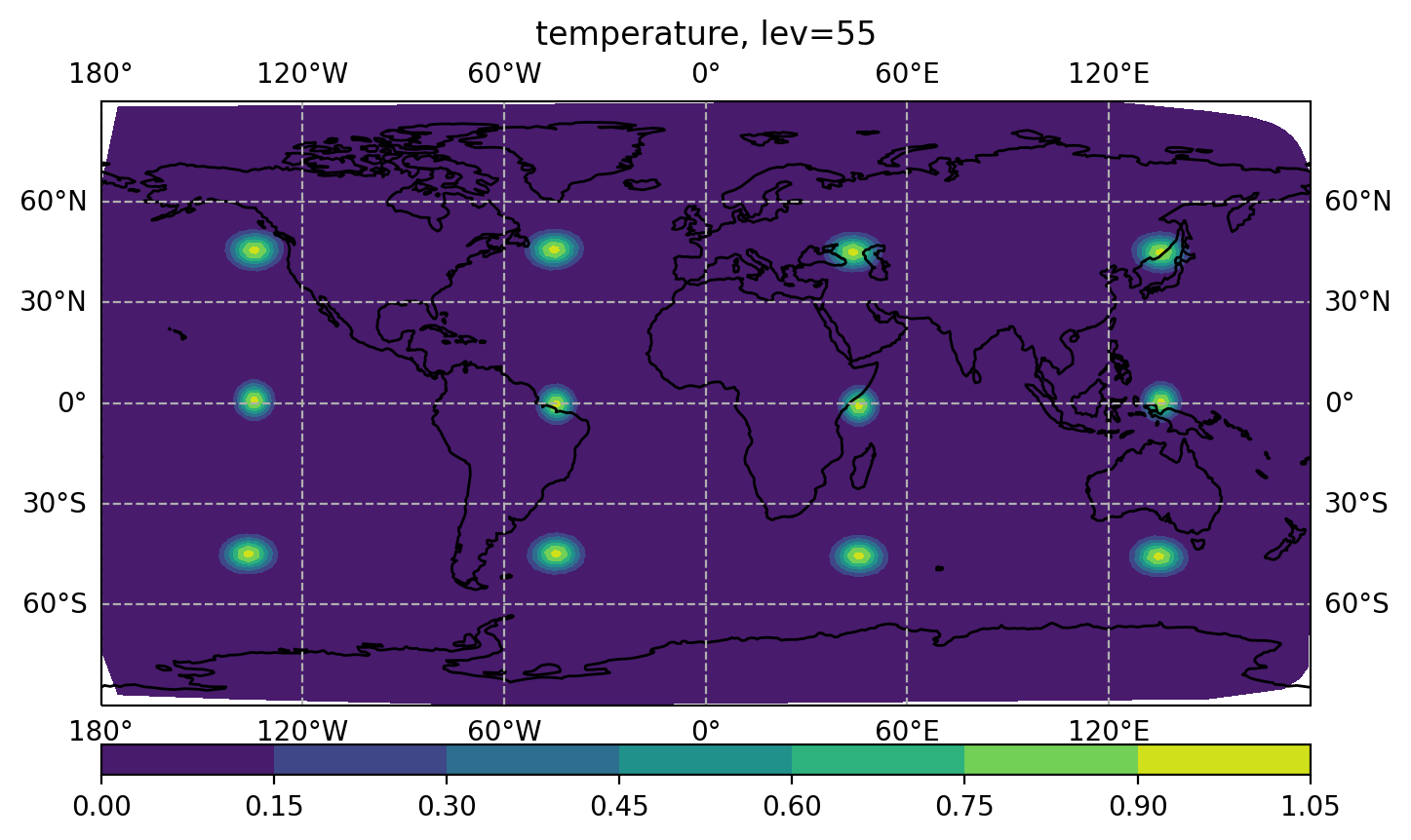
For a Dirac function multiplied by a given localization function, user can make a plot with dirac_nicas.2018-04-15_00.00.00.nc.
Copy the plotting script for Dirac output.
$ cp ../MPAS_JEDI_yamls_scripts/plot_bumploc.py ./
$ python plot_bumploc.py
$ module load imagemagick-7.0.8-7-gcc-11.2.0-46pk2go
$ display figure_bumploc.png

User can play with the specified localization lengths.
Please modify the following YAML keys from bumploc.yaml, then re-submit the SLURM job script.
[Note that dirac_nicas.2018-04-15_00.00.00.nc and
figure_bumploc.png will be overwritten, so it is a good idea
to rename the existing files to compare them to those from a new experiment with modified localization lengths.]
      ...
      io:
	files prefix: bumploc_1200km6km
      ...
      nicas:
        resolution: 8.0
        explicit length-scales: true
        horizontal length-scale:
          - groups: [common]
	    value: 1200.0e3
        vertical length-scale:
          - groups: [common]
	    value: 6.0e3
      ...
Make a plot for Dirac result (with plot_bumploc.py) to see how the localization looks like.
We are now ready to set up and run the first analysis test using 3DEnVar. For this 3DEnVar, we will use a 240 km background forecast and ensemble input at the same resolution.
Let's create a new working directory for this test:
$ cd /mnt/beegfs/${USER}/mpas_jedi_tutorial
$ mkdir 3denvar
$ cd 3denvar
Certifify that the enviroment variable is pointed by your mpas-bundle directory, giving the source the Spack-Stack-Araveck
$ . /mnt/beegfs/${USER}/mpas_jedi_tutorial/mpasbundlev3_local/build/SpackStackAraveck_intel_env_mpas_v8.2
The next commands in this section prepare the environment before the submit the job, which can be executed using the scripts commandos.ksh. Copy this script and running it.
$ cp /mnt/beegfs/luiz.sapucci/mpas_jedi_tutorial/3denvar/comandos.ksh .
$  ./comandos.ksh
Check and subit the sumit-file, but case you is not able to use this script, you should do the step-by-step below in this section.
We can then link the relevant MPAS stream, graph, namelist, and physics files:
$ ln -sf ../MPAS_namelist_stream_physics_files/*BL ./
$ ln -sf ../MPAS_namelist_stream_physics_files/*DATA ./
$ ln -sf ../MPAS_namelist_stream_physics_files/x1.10242.graph.info.part.64 ./
$ ln -sf ../MPAS_namelist_stream_physics_files/namelist.atmosphere_240km ./
$ ln -sf ../MPAS_namelist_stream_physics_files/streams.atmosphere_240km ./
$ ln -sf ../MPAS_namelist_stream_physics_files/stream_list*  ./
Next, we need to link in a few yaml files that define MPAS variables for JEDI:
$ ln -sf ${bundle_dir}/code/mpas-jedi/test/testinput/namelists/geovars.yaml ./
$ ln -sf ${bundle_dir}/code/mpas-jedi/test/testinput/namelists/keptvars.yaml ./
$ ln -sf ${bundle_dir}/code/mpas-jedi/test/testinput/obsop_name_map.yaml ./
Next, we need to link MPAS 2-stream files corresponding to 240 mesh.
For this experiment we need to link the following files:
$ ln -fs ../MPAS_namelist_stream_physics_files/x1.10242.invariant.nc .
$ ln -fs ../background/2018041418/mpasout.2018-04-15_00.00.00.nc ./templateFields.10242.nc
Next, we should link the background file mpasout.2018-04-15_00.00.00.nc into the working directory and make a copy of the background file as the analysis file to be overwritten.
$ ln -fs ../background/2018041418/mpasout.2018-04-15_00.00.00.nc ./bg.2018-04-15_00.00.00.nc
$ cp ../background/2018041418/mpasout.2018-04-15_00.00.00.nc ./an.2018-04-15_00.00.00.nc
Next, we need to link bump localization files.
$ ln -fs ../localization ./BUMP_files
Next, we need to link observation files into the working directory.
$ ln -fs ../obs_ioda_pregenerated/2018041500/aircraft_obs_2018041500.h5  .
$ ln -fs ../obs_ioda_pregenerated/2018041500/gnssro_obs_2018041500.h5  .
$ ln -fs ../obs_ioda_pregenerated/2018041500/satwind_obs_2018041500.h5  .
$ ln -fs ../obs_ioda_pregenerated/2018041500/sfc_obs_2018041500.h5  .
$ ln -fs ../obs_ioda_pregenerated/2018041500/sondes_obs_2018041500.h5  .
Next, we are ready to link the pre-prepared 3denvar.yaml file for 3DEnVar. 3denvar.yaml contains all of the settings we need for this 3DEnVar update.
$ ln -sf ../MPAS_JEDI_yamls_scripts/3denvar.yaml ./
We are finally ready to link a SLURM job script and then submit it. Notice that the job script runs an executable mpasjedi_variational.x, which is used for all of our variational updates.
$ cp ../MPAS_JEDI_yamls_scripts/run_3denvar.csh ./
It is need change the path of the $bundle_dir and comment the line to install Spack Stack, because is not necessary, change the partition to PESQ2
in the submit file run_3denvar.csh. In ordem to make easear this task copy this file as indicated bellow.
$ cp /mnt/beegfs/luiz.sapucci/mpas_jedi_tutorial/3denvar/run_3denvar.csh .
Certifify that the SpackStackAraveck is loaded and after submit a SLURM job to run hofx,
$  . /mnt/beegfs/${USER}/mpas_jedi_tutorial/mpasbundlev3_local/build/SpackStackAraveck_intel_env_mpas_v8.2
$  sbatch run_3denvar.csh
Once your job is submitted, you can check the status of the job using squeue -u ${USER}.
When the job is complete, you can check the log file by using vi mpasjedi_3denvar.log.
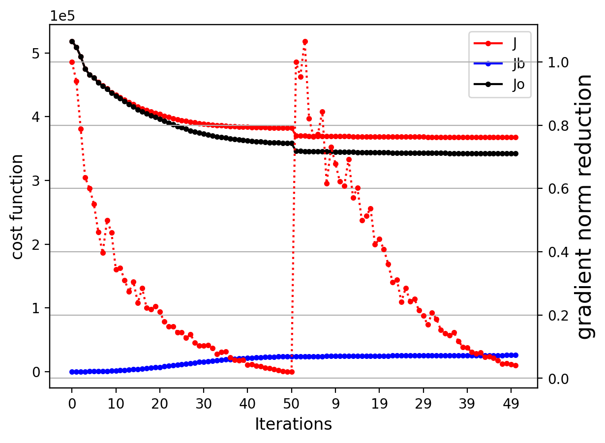
Now that the analysis was successful, you may plot the cost function and gradient norm reduction, for this setup conda environment for plotting.
Again, note that we need to load the conda environment before executing the Python script.
If you have already loaded the spack-stack modules, please open a new prompt before loading the conda environment 'mpasjedi'.
The important is that the spack-stack has not been loaded to use the mpasjedi env.
$  ssh -X username@egeon-login.cptec.inpe.br
$ cd /mnt/beegfs/${USER}/mpas_jedi_tutorial/localization
$ module load anaconda3-2022.05-gcc-11.2.0-q74p53i
$ source "/opt/spack/opt/spack/linux-rhel8-zen2/gcc-11.2.0/anaconda3-2022.05-q74p53iarv7fk3uin3xzsgfmov7rqomj/etc/profile.d/conda.sh"
$ conda activate /mnt/beegfs/professor/conda/envs/mpasjedi
Changing 'jedi.log' to 'mpasjedi_3denvar.log' in plot_cost_grad.py, then do
$ python plot_cost_grad.py
You can then view the figure using the following:
$ module load imagemagick-7.0.8-7-gcc-11.2.0-46pk2go
$ display costgrad.png

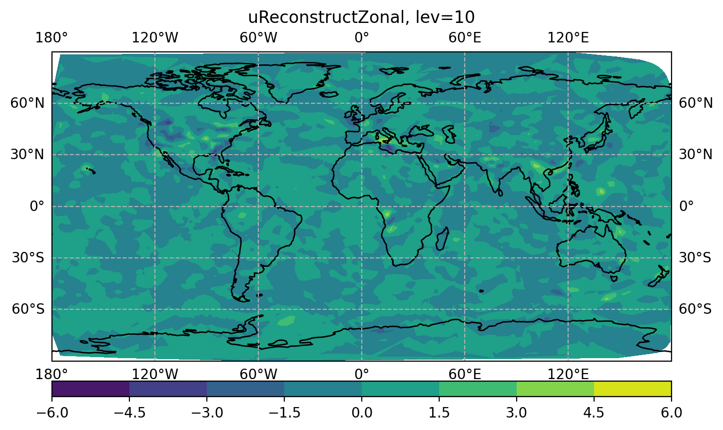
You can also plot the analysis increment (i.e., an.*.nc - bg.*.nc) with the following.
$  cp ../MPAS_JEDI_yamls_scripts/plot_analysis_increment.py ./
$  python plot_analysis_increment.py
$  display figure_increment_uReconstructZonal_10.png

You will also see several so-called DA "feedback" files below:
obsout_da_aircraft.h5
obsout_da_gnssro.h5
obsout_da_satwind.h5
obsout_da_sfc.h5
obsout_da_sondes.h5
You can follow the same procedure as in section 3.2 to plot these 'feedback' files, e.g.,
$ cp -r ${bundle_dir}/code/mpas-jedi/graphics .
$ cd graphics/standalone
$ python plot_diag.py
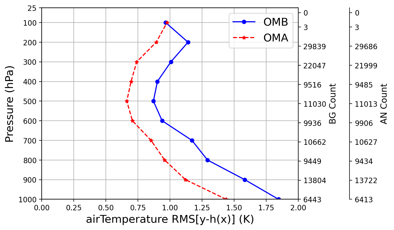
This will produce a number of figure files, display one of them
display RMSofOMM_da_aircraft_airTemperature.png
which will look like the figure below

Now we know how to run a 3DEnVar analysis, let's prepare a second test which uses a higher resolution background of 120 km but a coarser ensemble of 240 km.
Let's create a new working directory to run our 120-240km 3DEnVar update:
$ cd /mnt/beegfs/${USER}/mpas_jedi_tutorial
$ mkdir 3denvar_120km240km
$ cd 3denvar_120km240km
Certifify that the enviroment variable is pointed by your mpas-bundle directory, giving the source the Spack-Stack-Araveck
$ . /mnt/beegfs/${USER}/mpas_jedi_tutorial/mpasbundlev3_local/build/SpackStackAraveck_intel_env_mpas_v8.2
The next commands in this section prepare the environment before the submit the job, which can be executed using the scripts commandos.ksh. Copy this script and running it.
$ cp /mnt/beegfs/luiz.sapucci/mpas_jedi_tutorial/3denvar_120km240km/comandos.ksh .
$  ./comandos.ksh
Check and subit the sumit-file, but case you is not able to use this script, you should do the step-by-step below in this section before to do this.
We can then link the relevant MPAS stream, graph, namelist, and physics files. In addition to files for 240km mesh, we also need files for 120 km mesh.
$ ln -sf ../MPAS_namelist_stream_physics_files/*BL ./
$ ln -sf ../MPAS_namelist_stream_physics_files/*DATA ./
$ ln -sf ../MPAS_namelist_stream_physics_files/x1.10242.graph.info.part.64 ./
$ ln -sf ../MPAS_namelist_stream_physics_files/x1.40962.graph.info.part.64 ./
$ ln -sf ../MPAS_namelist_stream_physics_files/namelist.atmosphere_240km ./
$ ln -sf ../MPAS_namelist_stream_physics_files/namelist.atmosphere_120km ./
$ ln -sf ../MPAS_namelist_stream_physics_files/streams.atmosphere_240km ./
$ ln -sf ../MPAS_namelist_stream_physics_files/streams.atmosphere_120km ./
$ ln -sf ../MPAS_namelist_stream_physics_files/stream_list*  ./
Next, we need to link in a few yaml files again that define MPAS variables for JEDI:
$ ln -sf ${bundle_dir}/code/mpas-jedi/test/testinput/namelists/geovars.yaml ./
$ ln -sf ${bundle_dir}/code/mpas-jedi/test/testinput/namelists/keptvars.yaml ./
$ ln -sf ${bundle_dir}/code/mpas-jedi/test/testinput/obsop_name_map.yaml ./
Next, we need to link MPAS 2-stream files corresponding to both 240 km and 120 km MPAS grids. We need both invariant.nc file and templateFields.nc file.
For this experiment we need to link the following files:
$ ln -fs ../MPAS_namelist_stream_physics_files/x1.10242.invariant.nc .
$ ln -fs ../background/2018041418/mpasout.2018-04-15_00.00.00.nc ./templateFields.10242.nc
$ ln -fs ../MPAS_namelist_stream_physics_files/x1.40962.invariant.nc .
$ ln -fs ../background_120km/2018041418/mpasout.2018-04-15_00.00.00.nc ./templateFields.40962.nc
Next, we should link 120 km background file into the working directory and make a copy of the background file as the analysis file to be overwritten.
$ ln -fs ../background_120km/2018041418/mpasout.2018-04-15_00.00.00.nc ./bg.2018-04-15_00.00.00.nc
$ cp ../background_120km/2018041418/mpasout.2018-04-15_00.00.00.nc ./an.2018-04-15_00.00.00.nc
Next, we need to link our bump localization files.
$ ln -fs ../localization ./BUMP_files
Next, we need to link observation files into the working directory.
$ ln -fs ../obs_ioda_pregenerated/2018041500/aircraft_obs_2018041500.h5  .
$ ln -fs ../obs_ioda_pregenerated/2018041500/gnssro_obs_2018041500.h5  .
$ ln -fs ../obs_ioda_pregenerated/2018041500/satwind_obs_2018041500.h5  .
$ ln -fs ../obs_ioda_pregenerated/2018041500/sfc_obs_2018041500.h5  .
$ ln -fs ../obs_ioda_pregenerated/2018041500/sondes_obs_2018041500.h5  .
Next, we are ready to copy the pre-prepared 3denvar_120km240km.yaml file for this dual-resolution 3DEnVar.
$ ln -sf ../MPAS_JEDI_yamls_scripts/3denvar_120km240km.yaml ./3denvar.yaml
Copy a SLURM job script and revise it.
$ cp ../MPAS_JEDI_yamls_scripts/run_3denvar_dualres.sh ./
It is need change the path of the $bundle_dir and comment the line to install Spack Stack, because is not necessary, change the partition to PESQ2
in the submit file run_3denvar_dualres.sh. In ordem to make easear this task copy this file as indicated bellow.
$ cp /mnt/beegfs/luiz.sapucci/mpas_jedi_tutorial/3denvar_120km240km/run_3denvar_dualres.sh .
Certifify that the SpackStackAraveck is loaded and after submit a SLURM job to run 3denvar in dual resolution,
$  . /mnt/beegfs/${USER}/mpas_jedi_tutorial/mpasbundlev3_local/build/SpackStackAraveck_intel_env_mpas_v8.2
$  sbatch run_3denvar_dualres.sh
Note that this job script uses bash and a different mpas-bundle built under another build environment.
Again, you can check the status of the job using squeue -u ${USER}.
When the job is complete, you can check the log file by using vi mpasjedi_3denvar.log.
Again, you may plot cost function and gradient norm reduction as well as the analysis increment.
You need to change "x1.10242.invariant.nc" to "x1.40962.invariant.nc" within plot_analysis_increment.py in order to plot increment at the 120 km mesh.
Now we know how to run a 3DEnVar analysis, let's try 4DEnVar with 3 subwindows.
Let's create a new working directory to run 240km 4DEnVar:
$ cd /mnt/beegfs/${USER}/mpas_jedi_tutorial
$ mkdir 4denvar
$ cd 4denvar
Certifify that the enviroment variable is pointed by your mpas-bundle directory, giving the source the Spack-Stack-Araveck
$ . /mnt/beegfs/${USER}/mpas_jedi_tutorial/mpasbundlev3_local/build/SpackStackAraveck_intel_env_mpas_v8.2
The next commands in this section prepare the environment before the submit the job, which can be executed using the scripts commandos.ksh.
Copy this script and running it.
$ cp /mnt/beegfs/luiz.sapucci/mpas_jedi_tutorial/4denvar/comandos.ksh .
$  ./comandos.ksh
Check and subit the sumit-file, but case you is not able to use this script, you should do the step-by-step below in this section before to do this.
We can then link MPAS stream, graph, namelist, and physics files just as we did for 3DEnVar.
$ ln -sf ../MPAS_namelist_stream_physics_files/*BL ./
$ ln -sf ../MPAS_namelist_stream_physics_files/*DATA ./
$ ln -sf ../MPAS_namelist_stream_physics_files/x1.10242.graph.info.part.64 ./
$ ln -sf ../MPAS_namelist_stream_physics_files/namelist.atmosphere_240km ./
$ ln -sf ../MPAS_namelist_stream_physics_files/streams.atmosphere_240km ./
$ ln -sf ../MPAS_namelist_stream_physics_files/stream_list*  ./
Next, we need to link a few yaml files again that define MPAS variables for JEDI:
$ ln -sf ${bundle_dir}/code/mpas-jedi/test/testinput/namelists/geovars.yaml ./
$ ln -sf ${bundle_dir}/code/mpas-jedi/test/testinput/namelists/keptvars.yaml ./
$ ln -sf ${bundle_dir}/code/mpas-jedi/test/testinput/obsop_name_map.yaml ./
Next, we need to link MPAS 2-stream files corresponding to 240km mesh.
For this experiment we need to link the following files:
$ ln -fs ../MPAS_namelist_stream_physics_files/x1.10242.invariant.nc .
$ ln -fs ../background/2018041418/mpasout.2018-04-15_00.00.00.nc ./templateFields.10242.nc
Next, we need to link 240km background files for each subwindow into the working directory and make a copy of each background file as the analysis file for each subwindow to be overwritten.
$ ln -fs ../background/2018041418/mpasout.2018-04-14_21.00.00.nc ./bg.2018-04-14_21.00.00.nc
$ cp ../background/2018041418/mpasout.2018-04-14_21.00.00.nc     ./an.2018-04-14_21.00.00.nc
$ ln -fs ../background/2018041418/mpasout.2018-04-15_00.00.00.nc ./bg.2018-04-15_00.00.00.nc
$ cp ../background/2018041418/mpasout.2018-04-15_00.00.00.nc     ./an.2018-04-15_00.00.00.nc
$ ln -fs ../background/2018041418/mpasout.2018-04-15_03.00.00.nc ./bg.2018-04-15_03.00.00.nc
$ cp ../background/2018041418/mpasout.2018-04-15_03.00.00.nc     ./an.2018-04-15_03.00.00.nc
Next, we need to link bump localization files.
$ ln -fs ../localization ./BUMP_files
Next, we need to link observation files.
$ ln -fs ../obs_ioda_pregenerated/2018041500/aircraft_obs_2018041500.h5  .
$ ln -fs ../obs_ioda_pregenerated/2018041500/gnssro_obs_2018041500.h5  .
$ ln -fs ../obs_ioda_pregenerated/2018041500/satwind_obs_2018041500.h5  .
$ ln -fs ../obs_ioda_pregenerated/2018041500/sfc_obs_2018041500.h5  .
$ ln -fs ../obs_ioda_pregenerated/2018041500/sondes_obs_2018041500.h5  .
Next, we are ready to link the pre-prepared 4denvar.yaml file.
$ ln -sf ../MPAS_JEDI_yamls_scripts/4denvar.yaml ./4denvar.yaml
We are finally ready to link a job script and then submit a job. Note that this 4DEnVar job uses 3 nodes with 64 cores per node for 3 subwindows.
Copy a SLURM job script and revise it.
$ cp ../MPAS_JEDI_yamls_scripts/run_4denvar.csh ./
It is need change the path of the $bundle_dir and comment the line to install Spack Stack, because is not necessary, change the partition to PESQ2
in the submit file run_4denvar.csh. In ordem to make easear this task copy this file as indicated bellow.
$ cp /mnt/beegfs/luiz.sapucci/mpas_jedi_tutorial/4denvar/run_4denvar.csh .
Certifify that the SpackStackAraveck is loaded and after submit a SLURM job to run 3denvar in dual resolution,
$  . /mnt/beegfs/${USER}/mpas_jedi_tutorial/mpasbundlev3_local/build/SpackStackAraveck_intel_env_mpas_v8.2
$  sbatch run_4denvar.csh
Again, you can check the status of the job using qstat -u ${USER}.
When the job is complete, you can check the log file by using vi mpasjedi_4denvar.log.
Again, you can plot cost function and gradient norm reduction as well as analysis increments at one of 3 subwindows.
You may modify the an and bg files in plot_analysis_increment.py to see how the increment changes across the subwindows.
In this practice, we will run MPAS-JEDI 3DVar at global 240 km mesh.
The overall procedure is similar to the 3D/4DEnVar practice. However, 3DVar
uses the static multivariate background error covariance (B), which contains the
climatological characteristics. Here, the pre-generated static B will be used.
We hope to provide a practice for static B training in future MPAS-JEDI tutorials.
After changing to our /mnt/beegfs/${USER}/mpas_jedi_tutorial directory,
create the working directory for 3dvar.
$ cd /mnt/beegfs/${USER}/mpas_jedi_tutorial
$ mkdir 3dvar
$ cd 3dvar
Certifify that the enviroment variable is pointed by your mpas-bundle directory, giving the source the Spack-Stack-Araveck
$ . /mnt/beegfs/${USER}/mpas_jedi_tutorial/mpasbundlev3_local/build/SpackStackAraveck_intel_env_mpas_v8.2
The next commands in this section prepare the environment before the submit the job, which can be executed using the scripts commandos.ksh.
Copy this script and running it.
$ cp /mnt/beegfs/luiz.sapucci/mpas_jedi_tutorial/3dvar/comandos.ksh .
$  ./comandos.ksh
Check and subit the sumit-file, but case you is not able to use this script, you should do the step-by-step below in this section before to do this.
Link MPAS physics-related data and tables, MPAS graph, MPAS streams, and MPAS namelist files.
$ ln -fs ../MPAS_namelist_stream_physics_files/*BL ./
$ ln -fs ../MPAS_namelist_stream_physics_files/*DATA ./
$ ln -fs ../MPAS_namelist_stream_physics_files/x1.10242.graph.info.part.64 ./
$ ln -fs ../MPAS_namelist_stream_physics_files/streams.atmosphere_240km ./
$ ln -fs ../MPAS_namelist_stream_physics_files/stream_list.atmosphere.analysis ./
$ ln -fs ../MPAS_namelist_stream_physics_files/stream_list.atmosphere.background ./
$ ln -fs ../MPAS_namelist_stream_physics_files/stream_list.atmosphere.control ./
$ ln -fs ../MPAS_namelist_stream_physics_files/stream_list.atmosphere.ensemble ./
$ ln -fs ../MPAS_namelist_stream_physics_files/namelist.atmosphere_240km ./
Link the background file and copy it as an analysis file.
Note that mpas-jedi will overwrite
several selected analyzed variables (defined in stream_list.atmosphere.analysis)
in the analysis file.
$ ln -fs ../background/2018041418/mpasout.2018-04-15_00.00.00.nc ./bg.2018-04-15_00.00.00.nc
$ cp ./bg.2018-04-15_00.00.00.nc ./an.2018-04-15_00.00.00.nc
Link MPAS 2-stream files.
$ ln -fs ../MPAS_namelist_stream_physics_files/x1.10242.invariant.nc .
$ ln -fs ../background/2018041418/mpasout.2018-04-15_00.00.00.nc ./templateFields.10242.nc
Prepare the pre-generated static B files.
$ ln -fs ../B_Matrix ./
Create a directory for observation input, and link all the observation files to be assimilated.
Along with conventional observations, here a file for NOAA-18 AMSU-A radiance data is added.
$ ln -fs ../obs_ioda_pregenerated/2018041500/aircraft_obs_2018041500.h5  .
$ ln -fs ../obs_ioda_pregenerated/2018041500/gnssro_obs_2018041500.h5  .
$ ln -fs ../obs_ioda_pregenerated/2018041500/satwind_obs_2018041500.h5  .
$ ln -fs ../obs_ioda_pregenerated/2018041500/sfc_obs_2018041500.h5  .
$ ln -fs ../obs_ioda_pregenerated/2018041500/sondes_obs_2018041500.h5  .
$ ln -fs ../obs_ioda_pregenerated/2018041500/amsua_n18_obs_2018041500.h5 .
For this 3DVar test, satellite radiance data from an AMSU-A sensor is assimilated, so coefficient files for CRTM are needed.
$ ln -fs ../crtm_coeffs_v3 ./
Link yaml files:
$ ln -fs ${bundle_dir}/code/mpas-jedi/test/testinput/namelists/geovars.yaml  ./
$ ln -fs ${bundle_dir}/code/mpas-jedi/test/testinput/namelists/keptvars.yaml  ./
$ ln -fs ${bundle_dir}/code/mpas-jedi/test/testinput/obsop_name_map.yaml ./
$ ln -sf ../MPAS_JEDI_yamls_scripts/3dvar.yaml ./
Copy a SLURM job script and revise it.
$ cp ../MPAS_JEDI_yamls_scripts/run_3dvar.sh ./
It is need change the path of the $bundle_dir and comment the line to install Spack Stack, because is not necessary, change the partition to PESQ2
and build_sp to build in the submit file run_3dvar.sh. In ordem to make easear this task copy this file as indicated bellow.
$ cp /mnt/beegfs/luiz.sapucci/mpas_jedi_tutorial/3dvar/run_3dvar.sh .
Certifify that the SpackStackAraveck is loaded and after submit a SLURM job to run 3denvar in dual resolution,
$  . /mnt/beegfs/${USER}/mpas_jedi_tutorial/mpasbundlev3_local/build/SpackStackAraveck_intel_env_mpas_v8.2
$  sbatch run_3dvar.sh
As for section 4.3, this test case needs to use a different mpas-bundle built under another build environment.
User may check the SLURM job status by running squeue -u ${USER},
or monitoring the log file tail -f mpasjedi_3dvar.log .
User may want to try additional practice as below, e.g., Assimilate additional satellite radiances from another AMSU-A.
To do this, additional observation file (for example, ../obs_ioda_pregenerated/2018041500/amsua_n19_obs_2018041500.h5)
should be linked to /mnt/beegfs/${USER}/mpas_jedi_tutorial/3dvar/.
Also, user needs to add the corresponding obs space yaml key in 3dvar.yaml .
You should see some changes in fit-to-obs statistics, convergence, and analysis increment fields.
In this practice, we will run MPAS-JEDI Hybrid-3DEnVar at global 240 km mesh.
The hybrid covariance will be made from both static B and ensemble B.
After changing to /mnt/beegfs/${USER}/mpas_jedi_tutorial directory,
create the working directory for Hybrid-3DEnVar.
$ cd /mnt/beegfs/${USER}/mpas_jedi_tutorial
$ mkdir hybrid-3denvar
$ cd hybrid-3denvar
Certifify that the enviroment variable is pointed by your mpas-bundle directory, giving the source the Spack-Stack-Araveck
$ . /mnt/beegfs/${USER}/mpas_jedi_tutorial/mpasbundlev3_local/build/SpackStackAraveck_intel_env_mpas_v8.2
The next commands in this section prepare the environment before the submit the job, which can be executed using the scripts commandos.ksh.
Copy this script and running it.
$ cp /mnt/beegfs/luiz.sapucci/mpas_jedi_tutorial/hybrid-3denvar/comandos.ksh .
$  ./comandos.ksh
Check and subit the sumit-file, but case you is not able to use this script, you should do the step-by-step below in this section before to do this.
Link MPAS physics-related data and tables, MPAS graph, MPAS streams, and MPAS namelist files.
$ ln -fs ../MPAS_namelist_stream_physics_files/*BL ./
$ ln -fs ../MPAS_namelist_stream_physics_files/*DATA ./
$ ln -fs ../MPAS_namelist_stream_physics_files/x1.10242.graph.info.part.64 ./
$ ln -fs ../MPAS_namelist_stream_physics_files/streams.atmosphere_240km ./
$ ln -fs ../MPAS_namelist_stream_physics_files/stream_list.atmosphere.analysis ./
$ ln -fs ../MPAS_namelist_stream_physics_files/stream_list.atmosphere.background ./
$ ln -fs ../MPAS_namelist_stream_physics_files/stream_list.atmosphere.control ./
$ ln -fs ../MPAS_namelist_stream_physics_files/stream_list.atmosphere.ensemble ./
$ ln -fs ../MPAS_namelist_stream_physics_files/namelist.atmosphere_240km ./
Link the background file and copy it as an analysis file.
$ ln -fs ../background/2018041418/mpasout.2018-04-15_00.00.00.nc ./bg.2018-04-15_00.00.00.nc
$ cp ./bg.2018-04-15_00.00.00.nc ./an.2018-04-15_00.00.00.nc
Link MPAS 2-stream files.
$ ln -fs ../MPAS_namelist_stream_physics_files/x1.10242.invariant.nc .
$ ln -fs ../background/2018041418/mpasout.2018-04-15_00.00.00.nc ./templateFields.10242.nc
Prepare the pre-generated static B files.
$ ln -fs ../B_Matrix ./
Link the localization files.
$ ln -fs ../localization ./BUMP_files
Link all observation files to be assimilated.
$ ln -fs ../obs_ioda_pregenerated/2018041500/aircraft_obs_2018041500.h5  .
$ ln -fs ../obs_ioda_pregenerated/2018041500/gnssro_obs_2018041500.h5  .
$ ln -fs ../obs_ioda_pregenerated/2018041500/satwind_obs_2018041500.h5  .
$ ln -fs ../obs_ioda_pregenerated/2018041500/sfc_obs_2018041500.h5  .
$ ln -fs ../obs_ioda_pregenerated/2018041500/sondes_obs_2018041500.h5  .
$ ln -fs ../obs_ioda_pregenerated/2018041500/amsua_n18_obs_2018041500.h5 .
Prepare the coefficient files for CRTM.
$ ln -fs ../crtm_coeffs_v3 ./
Link yaml files.
$ ln -fs ${bundle_dir}/code/mpas-jedi/test/testinput/namelists/geovars.yaml  ./
$ ln -fs ${bundle_dir}/code/mpas-jedi/test/testinput/namelists/keptvars.yaml  ./
$ ln -fs ${bundle_dir}/code/mpas-jedi/test/testinput/obsop_name_map.yaml ./
$ ln -fs ../MPAS_JEDI_yamls_scripts/3dhyb.yaml ./
Copy a SLURM job script and revise it.
$ cp ../MPAS_JEDI_yamls_scripts/run_3dhyb.sh ./
It is need change the path of the $bundle_dir and comment the line to install Spack Stack, because is not necessary, change the partition to PESQ2
in the submit file run_3dhyb.sh. In ordem to make easear this task copy this file as indicated bellow.
$ cp /mnt/beegfs/luiz.sapucci/mpas_jedi_tutorial/hybrid-3denvar/run_3dhyb.sh .
Certifify that the SpackStackAraveck is loaded and after submit a SLURM job to run 3denvar hybrid,
$  . /mnt/beegfs/${USER}/mpas_jedi_tutorial/mpasbundlev3_local/build/SpackStackAraveck_intel_env_mpas_v8.2
$  sbatch run_3dhyb.sh
As section 4.3 and 5.1, this test case needs to use a different mpas-bundle built under another build environment.
User may check the job status by running squeue -u ${USER},
or monitoring the log file tail -f mpasjedi_3dhyb.log .
User may want to try addtional practice, e.g., change the hybrid weights.
The default 3dhyb.yaml uses 0.5 and 0.5 weights for static B and ensemble B. User can modify these weights, for example, 0.2/0.8 , 0.8/0.2 , 1.0/0.0 , 0.0/1.0 , or even 2.0/1.5 .
  background error:
    covariance model: hybrid
    components:
    - weight:
    value:  0.5
      covariance:
        covariance model: SABER
        ...
    - weight:
    value:  0.5
      covariance:
        covariance model: ensemble
        ...
You may see some changes in the fit-to-obs statistics, convergence, and analysis increment fields.
In this section, we will make plots for the statistics of OmB/OmA feedback files from two 2-day
cycling experiments by using the graphics package. In order to do this,
we first generate observation-space statistics following the instructions in Section 7.1,
then create the plots from statistics files following the instructions in Section 7.2.
The statistics are generated for each cycle and all ObsSpace (e.g., sondes, aircraft, gnssro, etc.) found in the folder containing the data assimilation feedback files (i.e., obsout_da_*.h5). The statistics are binned globally and by latitude bands as specified in config.py.
The binned statistics are stored in HDF5 files located in a folder named stats that is created for each cycle.
The statistics are generated by the script DiagnoseObsStatistics.py in graphics.
Let's begin by checking the directory omboma_from2experiments:
$ cd /mnt/beegfs/${USER}/mpas_jedi_tutorial/omboma_from2experiments
This folder contains sample variational-based DA observation "feedback" files from two experiments Exp1 and Exp2, e.g.,
$ ls Exp1/CyclingDA/*
You will see obsout_da_amsua_n18.h5 and obsout_da_gnssrobndropp1d.h5 under each cycle time during a 2-day period (9 cycles).
We can generate the bias, RMSE, and standard deviation statistics of these OMB/OMA files using
$  cp ../MPAS_JEDI_yamls_scripts/generate_stats_omboma.csh .
$ ln -sf ../MPAS_JEDI_yamls_scripts/advanceCYMDH.py .
It is need change the path of the $bundle_dir in two places in the script and comment the line to install Spack Stack, because is not necessary, change the partition to PESQ2
in the submit file generate_stats_omboma.csh. In ordem to make easear this task copy this file as indicated bellow.
$ cp /mnt/beegfs/luiz.sapucci/mpas_jedi_tutorial/omboma_from2experiments/generate_stats_omboma.csh .
Certifify that the SpackStackAraveck is loaded and after submit a SLURM job to run 3denvar hybrid,
$  . /mnt/beegfs/${USER}/mpas_jedi_tutorial/mpasbundlev3_local/build/SpackStackAraveck_intel_env_mpas_v8.2
$  sbatch generate_stats_omboma.csh
The job will take ~5 minutes to complete, and you can take a look at the folder of the statistics files:
$ ls Exp1/CyclingDA/*/stats
You will see two files stats_da_amsua_n18.h5 and stats_da_gnssrobndropp1d.h5 in each folder.
You may check generate_stats_omboma.csh, in which a line below generated statistical files.
python DiagnoseObsStatistics.py -n ${SLURM_NTASKS} -p ${daDiagDir} -o obsout -app variational -nout 1
where
-n: number of tasks/processors for multiprocessing (SLURM_NTASKS: number of tasks per node)
-p: path to DA feedback files (e.g., Exp1/CyclingDA/2018041500)
-o: prefix for DA feedback files
-app: application (variational or hofx)
-nout: number of outer loops
Also note that advanceCYMDH.py is a python code to help advance the time.
If statistics files were created, we can proceed to make the plots in the next section!
Again, note that we need to load the conda environment before executing the Python script.
If you have already loaded the spack-stack modules, please open a new prompt before loading the conda environment 'mpasjedi'.
The important is that the spack-stack has not been loaded to use the mpasjedi env.
$  ssh -X username@egeon-login.cptec.inpe.br
$ cd /mnt/beegfs/${USER}/mpas_jedi_tutorial/omboma_from2experiments
$ module load anaconda3-2022.05-gcc-11.2.0-q74p53i
$ source "/opt/spack/opt/spack/linux-rhel8-zen2/gcc-11.2.0/anaconda3-2022.05-q74p53iarv7fk3uin3xzsgfmov7rqomj/etc/profile.d/conda.sh"
$ conda activate /mnt/beegfs/professor/conda/envs/mpasjedi
Let us make a local copy of the graphics package first:
$ cd /mnt/beegfs/${USER}/mpas_jedi_tutorial/omboma_from2experiments
$ cp -r ${bundle_dir}/code/mpas-jedi/graphics .
$ cd graphics
Then do diff and replace analyze_config.py with a pre-prepared one:
$ diff analyze_config.py ../../MPAS_JEDI_yamls_scripts/analyze_config.py
$ mv analyze_config.py analyze_config.py_default
$ cp ../../MPAS_JEDI_yamls_scripts/analyze_config.py .
You can see the changes made in analyze_config.py by diff.
Below provides some explanations about settings in analyze_config.py.
- Set the first and last cycle date time:
dbConf['firstCycleDTime'] = dt.datetime(2018,4,15,0,0,0)
dbConf['lastCycleDTime'] = dt.datetime(2018,4,17,0,0,0)
- Set the time increment between valid date times to 6 hours:
dbConf['cyTimeInc'] = dt.timedelta(hours=6)
- Set the verification type to omb/oma:
VerificationType = 'omb/oma'
- Set the verification space to obs:
VerificationSpace = 'obs'
- Set the workflow type to MPAS-JEDI_tutorial:
workflowType = 'MPAS-JEDI_tutorial'
- Set the path to the experiment's folder:
dbConf['expDirectory'] = os.getenv('EXP_DIR','/mnt/beegfs/'+user+'/mpas_jedi_tutorial/omboma_from2experiments')
- Set the the name of the experiment that will be used as reference or control:
dbConf['cntrlExpName'] = 'exp1'
- Specify the experiments to be analyzed. Make sure that the value given to cntrlExpName is one of the keys in the dictionary experiments:
experiments['exp1'] = 'Exp1' + deterministicVerifyDir
experiments['exp2'] = 'Exp2' + deterministicVerifyDir
Last, setting python environment and running the script 'SpawnAnalyzeStats.py', but before that let's copy some needed files modified for Egeon machine:
$ mv JobScript.py JobScript.py_default
$ cp ../../MPAS_JEDI_yamls_scripts/JobScript.py .

$ mv SpawnAnalyzeStats.py SpawnAnalyzeStats.py_default
$ cp ../../MPAS_JEDI_yamls_scripts/SpawnAnalyzeStats.py .
Edit the script JobScript.py and change in the line 234 the partition to PESQ2. Finally do:
$ ./SpawnAnalyzeStats.py -app variational -nout 1 -d gnssrobndropp1d
$ ./SpawnAnalyzeStats.py -app variational -nout 1 -d amsua_n18
Each SpawnAnalyzeStats.py command triggers two SLURM jobs for making two types of
figures under gnssrobndropp1d_analyses and amsua_n18_analyses directories.
BinValAxisProfileDiffCI: vertical profiles of RMS relative differences from the RMS of OmB of Exp1 with confidence intervals (95%), as a function of the impact height for different latitude bands and binned by latitude at 10km
CYAxisExpLines: time series of the bias, count, RMS, and STD averaged globally and by latitude bands
SpawnAnalyzeStats.py can take some arguments (similar as in previous section), such as:
-app: application (e.g., variational, hofx)
-nout: number of outer loops in the variational method
-d: diagSpaces (e.g., amsua_,sonde,airc,sfc,gnssrobndropp1d,satwind)
You can check the status of the jobs using squeue -u ${USER}. Also, to monitor the progress of each job, you can check the 'an.log' file under the each analysis type directory, for example:
$ cd gnssrobndropp1d_analyses/CYAxisExpLines/omm
$ tail -f an.log
After jobs complete ('Finished main() successfully'), you may check gnssrobndropp1d_analyses/CYAxisExpLines/omm, for example,
$ cd gnssrobndropp1d_analyses/CYAxisExpLines/omm
$ module load imagemagick-7.0.8-7-gcc-11.2.0-46pk2go
$ display QCflag_good_TSeries_0min_gnssrobndropp1d_omm_RMS.pdf
which will look like the figure below

To view more figures, it is more convenent to transfer them to your local computer via:
$ scp -r ${USER}@egeon-login.cptec.inpe.br:/mnt/beegfs/${USER}/mpas_jedi_tutorial/omboma_from2experiments/graphics/gnssrobndropp1d_analyses .
$ scp -r ${USER}@egeon-login.cptec.inpe.br:/mnt/beegfs/${USER}/mpas_jedi_tutorial/omboma_from2experiments/graphics/amsua_n18_analyses .
